return
Thomas-Wigner rotation
In
special
relativity
the combination of two non-collinear pure
Lorentz
transformations (boosts)
is not a boost.
Rather, it is a boost combined with
a spatial rotation,
the
Thomas-Wigner
rotation.
We visualize this relativistic effect by moving a
Born-rigid
object
in two spatial dimensions (e.g. within the xy-plane)
on a closed trajectory.
For simplicity, the object's path is split into
a finite number of segments.
Within each segment the object's
proper
acceleration
is taken to be constant.
In addition to the acceleration's magnitude and direction
also the boost's (proper time) duration
is assumed to be the same in each section.
Finally,
the object is initially at rest
and
returns to its starting position
after completion of its trajectory.
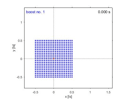
The animation above visualizes the
Thomas-Wigner
rotation
by boosting a square object
consisting 21 x 21 points
five times with a proper acceleration of 1 ls/s2.
Here, the unit of length is light-seconds (ls).
The color code indicates the individual point's
current segment number
(ranging from boost no. 1 to boost no. 5, top left).
Born-rigidity implies that the switchover
between
one boost segment to the next is synchronous
in the comoving
inertial
frame.
Hence, the switchover is
asynchronous in the
laboratory
frame
and at certain instances in (laboratory) time
one part of the object appears to be in one,
the other part in the next boost section.
This asynchronicity produces not only a shortening,
but also a shear effect,
which eventually adds up to the object's rotation.
The red point marks the reference vertex.
The clock in the top right corner
displays coordinate time in the laboratory frame.
The proper time duration for each boost is chosen
such that the objects lab frame velocity
is β = 0.7
at the end of boost no. 1.
With these parameter settings the resulting
Thomas-Wigner rotation angle is 33.7°.
This
movie
shows the same simulation
as the animinated GIF above,
however in higher resolution.
Technical details are given in
this paper.
The
SymPy
source files
vtwr3bst.py
and
vtwr5bst.py
are used in the derivation and evaluation
of several relations used in the simulation.
The
MATLAB
script
visualtwr.m
creates the simulation graphics.
References
M. Born (1909):
Die Theorie des starren Elektrons in der
Kinematik des Relativitätsprinzips.
Annalen der Physik, 335(11):1-56.
doi:10.1002/andp.19093351102
A. Einstein (1905):
Zur Elektrodynamik bewegter Körper.
Annalen der Physik, 322(10):891-921.
doi:10.1002/andp.19053221004
G. Herglotz (1909):
Über den vom Standpunkt des Relativitätsprinzips aus als
starr zu bezeichnenden Körper.
Annalen der Physik, 336(2):393-415.
doi:10.1002/andp.19103360208
F. Noether (1910):
Zur Kinematik des starren Körpers in der Relativtheorie.
Annalen der Physik, 336(5):919-944.
doi:10.1002/andp.19103360504
L. H. Thomas (1926):
The motion of the spinning electron.
Nature, 117(2945):514-514,
doi:10.1038/117514a0
L. H. Thomas (1927):
The kinematics of an electron with an axis.
Philos. Mag., 3(13):1-22,
doi:10.1080/14786440108564170
E. P. Wigner (1939):
On unitary representations of the inhomogeneous Lorentz group.
Ann. Math. 40(1):149-204,
doi:10.2307/1968551
return